I found a great open-source dataset Penn Haptic Adjective Corpus 2, and I want to learn/practice CNN-LSTM-Attention model on that dataset.
In this project, I explored the Penn Haptic Adjective Corpus 2 (PHAC-2) dataset. My goal was to build a Multimodal Deep Learning model that fuses visual data (images) with tactile sensor data (time-series) to classify physical properties of objects (e.g., “slippery,” “hard,” “fuzzy”).
Here is a walkthrough of how I implemented a CNN + Bi-LSTM + Attention architecture using PyTorch on Google Colab.
Environment & Data Preparation
The PHAC-2 dataset contains images of 60 objects and complex .h5 files recording robotic fingertip data.
Directly reading thousands of files from Google Drive is too slow for training. The first step is to mount Drive and unzip the dataset into the local Colab runtime (/content/local_data) to remove I/O bottlenecks 1.
import os

# 1. Mount Drive
from google.colab import drive
drive.mount('/content/drive')

# 2. Unzip to local runtime for speed
zip_path = '/content/drive/MyDrive/PHAC2_Project/dataset/doi-10.17617-3.0c79kw.zip' # Update with your path
extract_path = '/content/local_data'

if not os.path.exists(extract_path):
    os.makedirs(extract_path)
    !unzip -q "{zip_path}" -d "{extract_path}"
    print("Unzip finished!")
Data Engineering: The PHAC2Dataset Class
This was the most critical part of the project. The raw .h5 files use a nested group structure (e.g., biotacs/finger_0/...). We need to stitch different sensor channels together.
I created a custom Dataset class that:
-
Stitches Sensor Data: Concatenates
electrodes(19),pac(22),pdc(1),tac(1), andtdc(1) into a single 44-dimensional feature vector2. -
Downsamples: The raw sequences are ~13,000 steps long, which is overkill for an LSTM. I downsampled by a factor of 103.
-
Encodes Labels: dynamically builds a vocabulary of 24 adjectives and converts them to multi-hot vectors 4.
import torch
from torch.utils.data import Dataset, DataLoader
from torch.nn.utils.rnn import pad_sequence
import h5py
import os
import numpy as np
from PIL import Image
from torchvision import transforms

class PHAC2Dataset(Dataset):
    def __init__(self, h5_path, img_dir, transform=None, downsample_factor=10):
        """
        Args:
            h5_path: Path to .h5 file
            img_dir: Path to images folder
            transform: Image transforms
            downsample_factor: Take 1 frame every n frames to reduce sequence length (Critical for LSTM!)
        """
        self.h5_path = h5_path
        self.img_dir = img_dir
        self.transform = transform
        self.downsample_factor = downsample_factor

        # 1. First Pass: Scan file to find valid keys and build Label Vocabulary
        self.valid_keys = []
        self.all_adjectives = set() # Use a set to store unique adjectives

        print(f"Initializing Dataset... scanning H5 file for labels...")
        with h5py.File(self.h5_path, 'r') as f:
            for k in f.keys():
                # Check if it's a valid data sample (ends with digit)
                if k[-1].isdigit() and 'biotacs' in f[k]:
                    self.valid_keys.append(k)

                    # Collect adjectives for vocabulary
                    # Note: decoding bytes to string (b'cool' -> 'cool')
                    try:
                        labels = f[k]['adjectives'][:]
                        for label in labels:
                            self.all_adjectives.add(label.decode('utf-8'))
                    except:
                        pass # Some samples might miss labels

        self.valid_keys.sort()
        # Create mapping: 'cool' -> 0, 'hard' -> 1, ...
        self.adj_to_idx = {adj: i for i, adj in enumerate(sorted(list(self.all_adjectives)))}
        self.num_classes = len(self.adj_to_idx)

        print(f"Done! Found {len(self.valid_keys)} samples.")
        print(f"Found {self.num_classes} unique adjectives: {self.adj_to_idx}")

        # Cache image files for fast matching
        self.image_files = os.listdir(img_dir)

    def __len__(self):
        return len(self.valid_keys)

    def find_image(self, h5_key):
        # Key: 'acrylic_211_01' -> Unique ID: '211_01'
        parts = h5_key.split('_')
        unique_id = f"{parts[-2]}_{parts[-1]}"

        for img_file in self.image_files:
            if unique_id in img_file:
                return os.path.join(self.img_dir, img_file)
        return None

    def __getitem__(self, idx):
        key = self.valid_keys[idx]

        with h5py.File(self.h5_path, 'r') as f:
            # --- 1. Load Tactile Data ---
            # Path: biotacs -> finger_0 -> [electrodes, pac, pdc, tac, tdc]
            try:
                finger_0 = f[key]['biotacs']['finger_0']

                # Load and reshape 1D arrays to (T, 1)
                electrodes = finger_0['electrodes'][:] # (T, 19)
                pac = finger_0['pac'][:]               # (T, 22)
                pdc = finger_0['pdc'][:] [:, np.newaxis] # (T,) -> (T, 1)
                tac = finger_0['tac'][:] [:, np.newaxis] # (T, 1)
                tdc = finger_0['tdc'][:] [:, np.newaxis] # (T, 1)

                # Concatenate all features: 19+22+1+1+1 = 44 features
                # Axis 1 is the feature dimension
                raw_data = np.concatenate([electrodes, pac, pdc, tac, tdc], axis=1)

                # Downsample (Simple slicing)
                # raw_data[::10] means take every 10th element
                downsampled_data = raw_data[::self.downsample_factor]

                # Convert to Float Tensor and Normalize roughly (divide by large number or standard scaling)
                # Raw sensor data can be large integers, better to scale them slightly for LSTM stability
                # For now, just casting to float is enough to run.
                biotac_tensor = torch.tensor(downsampled_data, dtype=torch.float32)

            except Exception as e:
                print(f"Error loading sensor data for {key}: {e}")
                # Return dummy zeros if failed
                biotac_tensor = torch.zeros((100, 44))

            # --- 2. Load Labels (Multi-hot Encoding) ---
            label_vector = torch.zeros(self.num_classes, dtype=torch.float32)
            try:
                raw_labels = f[key]['adjectives'][:]
                for l in raw_labels:
                    l_str = l.decode('utf-8')
                    if l_str in self.adj_to_idx:
                        idx = self.adj_to_idx[l_str]
                        label_vector[idx] = 1.0
            except:
                pass # No labels

        # --- 3. Load Image ---
        img_path = self.find_image(key)
        if img_path:
            image = Image.open(img_path).convert('RGB')
        else:
            image = Image.new('RGB', (224, 224), color='black')

        if self.transform:
            image = self.transform(image)

        return biotac_tensor, image, label_vector

# --- Collate Function ---
def my_collate_fn(batch):
    biotacs, images, labels = zip(*batch)
    biotacs_padded = pad_sequence(biotacs, batch_first=True, padding_value=0.0)
    images_stacked = torch.stack(images)
    labels_stacked = torch.stack(labels)
    return biotacs_padded, images_stacked, labels_stacked

# --- Run Test ---
# Setup Transforms
img_transforms = transforms.Compose([
    transforms.Resize((224, 224)),
    transforms.ToTensor(),
    transforms.Normalize(mean=[0.485, 0.456, 0.406], std=[0.229, 0.224, 0.225])
])

# Paths
h5_path = '/content/local_data/phac_train_test_pos_neg_90_10_1_20.h5'
img_dir = '/content/local_data/Images'

# Create Dataset (using downsample_factor=10 to reduce sequence length from 13000 to 1300)
dataset = PHAC2Dataset(h5_path, img_dir, transform=img_transforms, downsample_factor=10)

# Create DataLoader
dataloader = DataLoader(dataset, batch_size=4, shuffle=True, collate_fn=my_collate_fn)

# Check one batch
print("\n=== Data Loading Test ===")
tactile, imgs, lbls = next(iter(dataloader))
print(f"Tactile Shape (Batch, Time, Feat): {tactile.shape}")
print(f"Image Shape   (Batch, C, H, W):    {imgs.shape}")
print(f"Label Shape   (Batch, Classes):    {lbls.shape}")

# Verify Feature Dimension
assert tactile.shape[2] == 44, f"Error: Expected 44 features, got {tactile.shape[2]}"
print("✅ Feature dimension is correct: 44")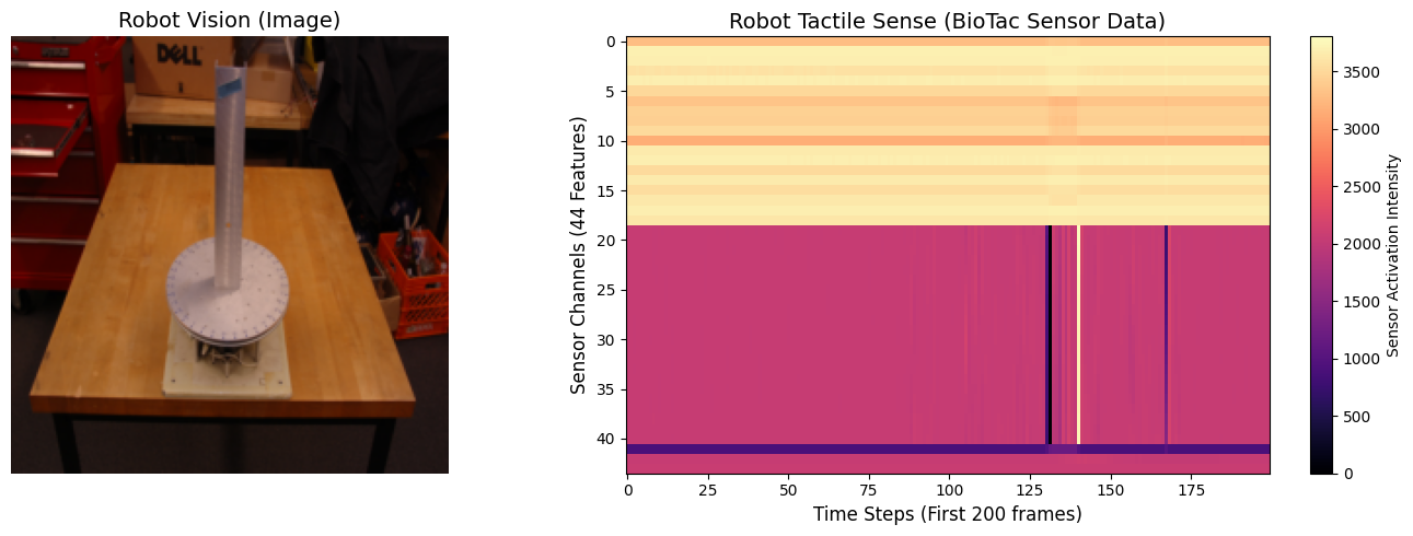
The Architecture: VisuoTactileNet
I designed a two-stream network.
The Attention Mechanism:
Tactile data is temporal—the most important information might happen in a split second (like the initial contact). I implemented a Self-Attention mechanism to let the LSTM focus on specific time steps 5.
The Fusion:
- Visual Branch: A pretrained ResNet18 (minus the top layer).
- Tactile Branch: A Bidirectional LSTM (Hidden Size 128) -> Attention.
- Fusion: Concatenation of the visual (256 dim) and tactile (256 dim) vectors.
import torch.nn as nn
import torchvision.models as models
import torch.nn.functional as F

class Attention(nn.Module):
    def __init__(self, hidden_dim):
        super(Attention, self).__init__()
        self.attention_weights = nn.Linear(hidden_dim, 1)

    def forward(self, lstm_output):
        # lstm_output: (Batch, Time, Hidden)
        scores = self.attention_weights(lstm_output)
        alpha = F.softmax(scores, dim=1)
        # Weighted sum (Context Vector)
        context = torch.sum(lstm_output * alpha, dim=1)
        return context, alpha

class VisuoTactileNet(nn.Module):
    def __init__(self, num_classes=24, tactile_input_dim=44, lstm_hidden_dim=128):
        super(VisuoTactileNet, self).__init__()

        # A. Visual Branch (ResNet18)
        resnet = models.resnet18(pretrained=True)
        self.visual_encoder = nn.Sequential(*list(resnet.children())[:-1])
        self.visual_fc = nn.Linear(512, 256)

        # B. Tactile Branch (Bi-LSTM + Attention)
        self.lstm = nn.LSTM(input_size=tactile_input_dim,
                            hidden_size=lstm_hidden_dim,
                            num_layers=1,
                            batch_first=True,
                            bidirectional=True)
        self.attention = Attention(lstm_hidden_dim * 2)

        # C. Fusion Classifier
        fusion_dim = 256 + (lstm_hidden_dim * 2)
        self.classifier = nn.Sequential(
            nn.Linear(fusion_dim, 128),
            nn.ReLU(),
            nn.Dropout(0.3),
            nn.Linear(128, num_classes)
        )

    def forward(self, tactile_seq, images):
        # Visual
        v_feat = self.visual_encoder(images)
        v_feat = v_feat.view(v_feat.size(0), -1)
        v_feat = F.relu(self.visual_fc(v_feat))

        # Tactile
        lstm_out, _ = self.lstm(tactile_seq)
        t_feat, attn_weights = self.attention(lstm_out)

        # Fusion
        combined = torch.cat((v_feat, t_feat), dim=1)
        return self.classifier(combined), attn_weights
Training Loop
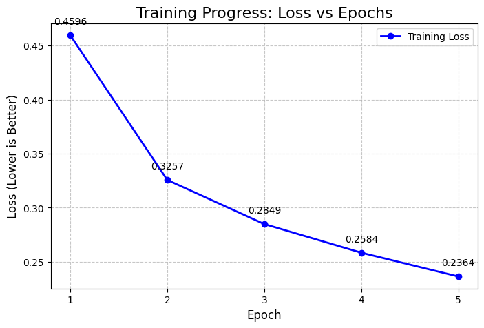
This is a multi-label classification problem (an object can be both “hard” and “smooth”), so I used BCEWithLogitsLoss. I ran this for 5 epochs on the T4 GPU.
import torch.optim as optim
from tqdm import tqdm

# Hyperparameters
device = torch.device("cuda" if torch.cuda.is_available() else "cpu")
model = VisuoTactileNet(num_classes=24).to(device)
criterion = nn.BCEWithLogitsLoss()
optimizer = optim.Adam(model.parameters(), lr=1e-4)

# Training Loop
num_epochs = 5
for epoch in range(num_epochs):
    model.train()
    running_loss = 0.0
    progress_bar = tqdm(dataloader, desc=f"Epoch {epoch+1}/{num_epochs}")

    for batch_tactile, batch_images, batch_labels in progress_bar:
        batch_tactile = batch_tactile.to(device)
        batch_images = batch_images.to(device)
        batch_labels = batch_labels.to(device)

        optimizer.zero_grad()
        logits, _ = model(batch_tactile, batch_images)
        loss = criterion(logits, batch_labels)

        loss.backward()
        optimizer.step()

        running_loss += loss.item()
        progress_bar.set_postfix({'loss': running_loss / (progress_bar.n + 1)})

    print(f"Epoch {epoch+1} Complete! Average Loss: {running_loss / len(dataloader):.4f}")
The training converged well, with the loss dropping from 0.4596 in Epoch 1 to 0.2364 in Epoch 56666.
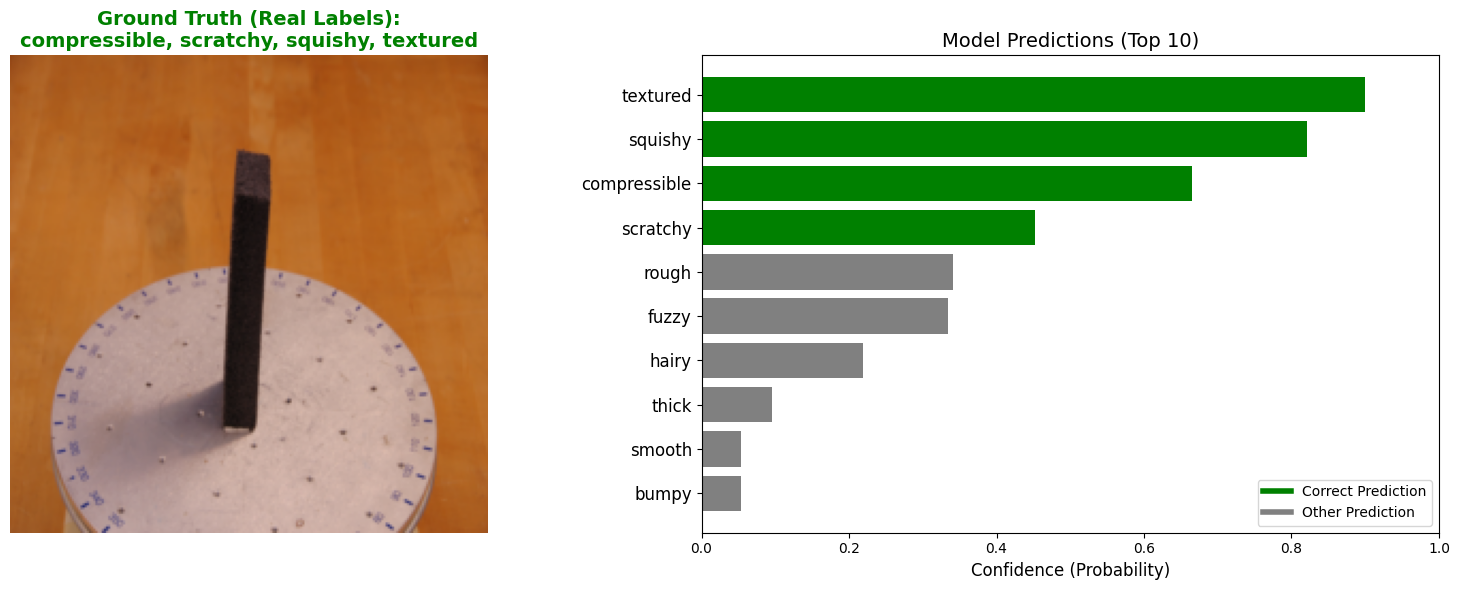
Inference & Results
To visualize the model’s performance, I grabbed a validation sample and compared the model’s top predictions against the ground truth.
import matplotlib.pyplot as plt
import numpy as np

tactile, image, label = dataset[10]

fig, ax = plt.subplots(1, 2, figsize=(15, 5))

img_np = image.permute(1, 2, 0).numpy()

mean = np.array([0.485, 0.456, 0.406])
std = np.array([0.229, 0.224, 0.225])
img_np = std * img_np + mean
img_np = np.clip(img_np, 0, 1)

ax[0].imshow(img_np)
ax[0].set_title("Robot Vision (Image)", fontsize=14)
ax[0].axis('off')

tactile_map = tactile.t().numpy()

im = ax[1].imshow(tactile_map[:, :200], aspect='auto', cmap='magma', interpolation='nearest')
ax[1].set_title("Robot Tactile Sense (BioTac Sensor Data)", fontsize=14)
ax[1].set_xlabel("Time Steps (First 200 frames)", fontsize=12)
ax[1].set_ylabel("Sensor Channels (44 Features)", fontsize=12)
plt.colorbar(im, ax=ax[1], label="Sensor Activation Intensity")

plt.tight_layout()
plt.show()
epochs = [1, 2, 3, 4, 5]
losses = [0.4596, 0.3257, 0.2849, 0.2584, 0.2364]
plt.figure(figsize=(8, 5))
plt.plot(epochs, losses, marker='o', linestyle='-', color='b', linewidth=2, label='Training Loss')
plt.title("Training Progress: Loss vs Epochs", fontsize=16)
plt.xlabel("Epoch", fontsize=12)
plt.ylabel("Loss (Lower is Better)", fontsize=12)
plt.grid(True, linestyle='--', alpha=0.7)
plt.xticks(epochs)
plt.legend()
for x, y in zip(epochs, losses):
plt.text(x, y + 0.01, f"{y:.4f}", ha='center', fontsize=10)
plt.show()import torch.nn.functional as F
model.eval()
data_iter = iter(dataloader)
tactile_batch, img_batch, label_batch = next(data_iter)
sample_idx = 0
input_tactile = tactile_batch[sample_idx].unsqueeze(0).to(device)
input_image = img_batch[sample_idx].unsqueeze(0).to(device)
true_label = label_batch[sample_idx]
with torch.no_grad():
logits, _ = model(input_tactile, input_image)
probs = torch.sigmoid(logits)
probs = probs.cpu().squeeze().numpy()
idx_to_adj = {v: k for k, v in dataset.adj_to_idx.items()}
all_adjectives = [idx_to_adj[i] for i in range(len(probs))]
fig, ax = plt.subplots(1, 2, figsize=(16, 6))
img_display = input_image.cpu().squeeze().permute(1, 2, 0).numpy()
img_display = std * img_display + mean
img_display = np.clip(img_display, 0, 1)
ax[0].imshow(img_display)
true_indices = torch.where(true_label == 1)[0].numpy()
true_words = [idx_to_adj[i] for i in true_indices]
title_text = "Ground Truth (Real Labels):\n" + ", ".join(true_words)
ax[0].set_title(title_text, fontsize=14, color='green', fontweight='bold')
ax[0].axis('off')
top_n = 10
top_indices = probs.argsort()[-top_n:][::-1]
top_probs = probs[top_indices]
top_words = [all_adjectives[i] for i in top_indices]
colors = ['green' if word in true_words else 'gray' for word in top_words]
y_pos = np.arange(len(top_words))
ax[1].barh(y_pos, top_probs, align='center', color=colors)
ax[1].set_yticks(y_pos)
ax[1].set_yticklabels(top_words, fontsize=12)
ax[1].invert_yaxis()
ax[1].set_xlabel('Confidence (Probability)', fontsize=12)
ax[1].set_title('Model Predictions (Top 10)', fontsize=14)
ax[1].set_xlim(0, 1.0)
from matplotlib.lines import Line2D
legend_elements = [Line2D([0], [0], color='green', lw=4, label='Correct Prediction'),
Line2D([0], [0], color='gray', lw=4, label='Other Prediction')]
ax[1].legend(handles=legend_elements)
plt.tight_layout()
plt.show()